Digital Audio Basics: Stair Steps and Sample Rates

I took a prior stab at discussing vinyl versus digital audio, and I want to do a better job, but it’s going to take a bit of background discussion first.  I feel that to have an understanding of digital audio, and to discuss comparisons between say Vinyl and CD, or CD and high resolution audio, the concepts of sample rate and sample bits in digital audio need to be explored first.

I’m both excited and embarrassed to be writing this post.  I’m not Joe on the street, many years ago I took classes in digital signal and image processing, I earned graduate degrees in engineering from a prestigious university (although it has been a few years….), and yet I realize I didn’t have an intuitive grasp of some basic concepts.

I find that for myself, and for many others, concepts around digital images are more intuitive than concepts around digital audio.  For digital images, most of us know that a digital image is composed of little squares or pixels, each pixel is a single color, and the more the pixels the better the picture.  The color accuracy of a pixel is determined by the number of binary digits (bits) – the more the bits, the finer the gradation of a color from light to dark. A digital audio file is a lot like a digital image file, except that a digital image file has color data for points in space (the pixels), and a digital audio file has signal data (corresponding to the sound level) for points in time.  With digital audio, we have sound samples (corresponding to pixels), and binary data (bits) that determine the gradation of sound from soft to loud.

Most of us expect that, in audio, we get closer to the original signal by having more samples and more bits.  There are two issues that make our intuition not fully correct.  The first issue is the limited range of human hearing, and the second issue is the presence of noise, both naturally in our environment, and in all recorded audio.

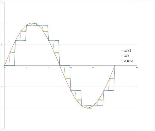
First I’m going to talk about sampling rate, or how many audio samples are collected say every second.  The second issue, how much data (bits) is stored with each simple, will be considered in a separate post.  Let’s consider what happens when we sample a pure tone, say a sine wave.  Here I am not concerned with the precision of the sample, so we are not thinking about measurement error, round off error, or “quantization” that happens from using a finite amount of data to capture each sample.  Many readers will likely have seen a graph like below; suppose the smooth red curve is the original signal, the blue “stepped” curve shows the digitized version with say 10 samples, and the light green “stepped” curve shows the digitized version with say 20 samples.

A graph like the one above is a source of a lot of wrong thinking about digital signals.  What the above implies is that 10 samples gives a crude approximation of the original signal, 20 samples gives a better but still crude approximation, and that if we continued to increase the number of samples we would eventually get to a pretty good approximation of the original signal.  But this is completely wrong!

There is a famous theorem, the Nyquist-Shannon sampling theorem, and I recently realized (courtesy of a video from Xiph.org), that I didn’t truly grasp it.  What the Nyquist-Shannon sample theorem says is that if the frequency content of the original signal is limited to some maximum, say M (e.g., say 20KHz for human hearing), and if we collect samples at frequency 2M, then we can perfectly reconstruct the original signal.  In the example above, then, going from 10 samples to 20 samples does nothing to improve the accuracy of the reconstructed signal, as the original signal was a pure sine wave  and with 10 samples we are already way over the minimum of twice the frequency of the original signal.

So why does it go against intuition to think that more digital samples means a closer approximation of the original signal?  Probably because (most of us) we tend to mentally think of a stair step reconstruction of the original signal from the samples! Where do the stair steps come from?  From the idea of sample and hold.  Remember, a sample is the signal value at a particular time, but we don’t know (or record) the signal value in between samples.  So the simple thing to do is just imagine that the signal does not change values between samples, which is how I drew the above graph.

The reconstruction of an analog audio signal from digital samples though, does not use sample and hold for the final result.  The conversion process is more like a kind of curve fitting, requiring there to be a smooth output that goes through the sampled values.  If there were sudden stair step jumps in the reproduced signal, those sudden jumps would have high frequency content beyond our maximum frequency M.

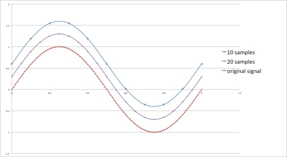
To demonstrate, and this is not any sort of rigorous proof, but a way to improve intuition, I used Microsoft Excel, and I created 3 data sets for a sine wave: the first data set (red) represents the original signal (actually with 100 points), then 20 sample points, then 10 sample points.  I displaced the curves vertically so it is easy to see, they all have the exact same shape, and that is what happens when a digital audio file is reconstructed to be an analog signal – one gets a smooth signal with no stair steps, and increasing the number of samples does not improve the smoothness of the final signal:

Again, for most of us, this result is highly counter intuitive – surely more samples must make for a smoother curve.  The point though is that we have taken samples of a bandwidth limited signal – a signal that has maximum frequency content M.  If there was something “unsmooth” or highly irregular looking going on between the samples, that would imply higher frequency content.  Since we are sampling at 2M or greater, we have captured enough information even with the “crude” 10 samples.

Said another way, if I had not displaced the three curves vertically, they would lie exactly atop each other, and THAT is what the Nyquist-Shannon sampling theorem states: we can exactly reconstruct the original signal from the sampled data provided we have sufficient samples, and sufficient for this example would be only 2 samples!

A brilliant demonstration of the above is given by Monty Montgomery in the following video:

http://xiph.org/video/vid2.shtml

or on youtube at

Now one question in my mind, and perhaps yours, is what about measurement error and measurement precision?  I recall taking a basic lab course many years ago, and one of the first things drilled in to me (not talking about digital audio here) is that all measurements have limited accuracy.  Suppose I want to use a ruler and measure the length of a piece of paper.  The ruler has tick marks say every millimeter, or every 1/16 of an inch, so that limits the precision of my measurements.  Not only does the ruler have limited accuracy, if I make multiple measurements, or if more than one person makes measurements, it is unlikely that we get the same value every time.

In a future post, I’ll touch on the issue of measurement error and use Microsoft Excel to create a simple spreadsheet and graph the effect of timing errors (recording a sample say at .1003 seconds instead of exactly at .1 seconds), and the effect of using varying measurement precision (more or less bits) for the samples.

Thanks for reading!